Multi-step-ahead NARX model

In this example, we will compare one-step-ahead NARX and multi-step-ahead NARX.

# Authors: The fastcan developers
# SPDX-License-Identifier: MIT

Nonlinear system

Duffing equation is used to generate simulated data. The mathematical model is given by

\[\ddot{y} + 0.1\dot{y} - y + 0.25y^3 = u\]

where \(y\) is the output signal and \(u\) is the input signal, which is \(u(t) = 2.5\cos(2\pi t)\).

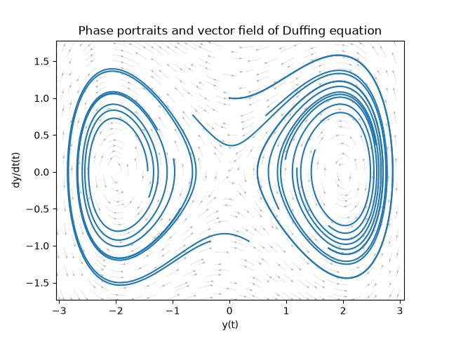
The phase portraits and the vector field of the Duffing equation are shown below.

import matplotlib.pyplot as plt
import numpy as np
from scipy.integrate import odeint


def duffing_equation(y, t):
    """Non-autonomous system"""
    # y1 is displacement and y2 is velocity
    y1, y2 = y
    # u is sinusoidal input
    u = 2.5 * np.cos(2 * np.pi * t)
    # dydt is derivative of y1 and y2
    dydt = [y2, -0.1 * y2 + y1 - 0.25 * y1**3 + u]
    return dydt


def auto_duffing_equation(y, t):
    """Autonomous system"""
    y1, y2 = y
    dydt = [y2, -0.1 * y2 + y1 - 0.25 * y1**3]
    return dydt


dur = 10
n_samples = 1000

y0 = None
if y0 is None:
    n_init = 10
    x0 = np.linspace(0, 2, n_init)
    y0_y = np.cos(np.pi * x0)
    y0_x = np.sin(np.pi * x0)
    y0 = np.c_[y0_x, y0_y]
else:
    n_init = len(y0)

t = np.linspace(0, dur, n_samples)
sol = np.zeros((n_init, n_samples, 2))
for i in range(n_init):
    sol[i] = odeint(auto_duffing_equation, y0[i], t)

# Phase portraits
for i in range(n_init):
    plt.plot(sol[i, :, 0], sol[i, :, 1], c="tab:blue")

# Vector field
y_min = np.min(sol[:, :, 0]) - 0.2
y_max = np.max(sol[:, :, 0]) + 0.2
dot_y_min = np.min(sol[:, :, 1]) - 0.2
dot_y_max = np.max(sol[:, :, 1]) + 0.2
y, dot_y = np.meshgrid(
    np.linspace(y_min, y_max, 30), np.linspace(dot_y_min, dot_y_max, 30)
)
ddot_y = auto_duffing_equation([y, dot_y], 0)[1]
plt.streamplot(
    y,
    dot_y,
    dot_y,
    ddot_y,
    color=(0.5, 0.5, 0.5, 0.3),
    density=1.5,
    minlength=0.02,
    maxlength=0.1,
    linewidth=0.5,
    arrowsize=0.5,
)

plt.xlim(y_min, y_max)
plt.ylim(dot_y_min, dot_y_max)
plt.title("Phase portraits and vector field of Duffing equation")
plt.xlabel("y(t)")
plt.ylabel("dy/dt(t)")
plt.show()

Generate training-test data

In the phase portraits, it is shown that the system has two stable equilibria. We use one to generate training data and the other to generate test data.

# 10 s duration with 0.01 Hz sampling time,
# so 1000 samples in total for each measurement
dur = 10
n_samples = 1000
t = np.linspace(0, dur, n_samples)
# External excitation is the same for each measurement
u = 2.5 * np.cos(2 * np.pi * t).reshape(-1, 1)

# Small additional white noise
rng = np.random.default_rng(12345)
e_train_0 = rng.normal(0, 0.0004, n_samples)
e_test = rng.normal(0, 0.0004, n_samples)

# Solve differential equation to get displacement as y
# Initial condition at displacement 0.6 and velocity 0.8
sol = odeint(duffing_equation, [0.6, 0.8], t)
y_train_0 = sol[:, 0] + e_train_0

# Initial condition at displacement 0.6 and velocity -0.8
sol = odeint(duffing_equation, [0.6, -0.8], t)
y_test = sol[:, 0] + e_test

One-step-head VS. multi-step-ahead NARX

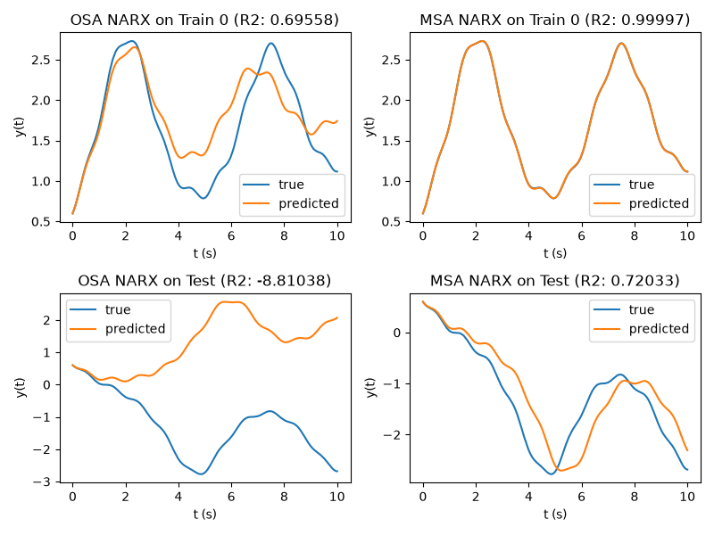
First, we use make_narx() to obtain the reduced NARX model. Then, the NARX model will be fitted with one-step-ahead predictor and multi-step-ahead predictor, respectively. Generally, the training of one-step-ahead (OSA) NARX is faster, while the multi-step-ahead (MSA) NARX is more accurate.

from sklearn.metrics import r2_score

from fastcan.narx import make_narx

max_delay = 3

narx_model = make_narx(
    X=u,
    y=y_train_0,
    n_terms_to_select=5,
    max_delay=max_delay,
    poly_degree=3,
    verbose=0,
)


def plot_prediction(ax, t, y_true, y_pred, title):
    ax.plot(t, y_true, label="true")
    ax.plot(t, y_pred, label="predicted")
    ax.legend()
    ax.set_title(f"{title} (R2: {r2_score(y_true, y_pred):.5f})")
    ax.set_xlabel("t (s)")
    ax.set_ylabel("y(t)")


# OSA NARX
narx_model.fit(u, y_train_0)
y_train_0_osa_pred = narx_model.predict(u, y_init=y_train_0[:max_delay])
y_test_osa_pred = narx_model.predict(u, y_init=y_test[:max_delay])

# MSA NARX
narx_model.fit(u, y_train_0, coef_init="one_step_ahead")
y_train_0_msa_pred = narx_model.predict(u, y_init=y_train_0[:max_delay])
y_test_msa_pred = narx_model.predict(u, y_init=y_test[:max_delay])

fig, ax = plt.subplots(2, 2, figsize=(8, 6))
plot_prediction(ax[0, 0], t, y_train_0, y_train_0_osa_pred, "OSA NARX on Train 0")
plot_prediction(ax[0, 1], t, y_train_0, y_train_0_msa_pred, "MSA NARX on Train 0")
plot_prediction(ax[1, 0], t, y_test, y_test_osa_pred, "OSA NARX on Test")
plot_prediction(ax[1, 1], t, y_test, y_test_msa_pred, "MSA NARX on Test")
fig.tight_layout()
plt.show()

Multiple measurement sessions

The plot above shows that the NARX model cannot capture the dynamics at the left equilibrium shown in the phase portraits. To improve the performance, let us append another measurement session to the training data to include the dynamics of both equilibria. Here, we need to insert (at least max_delay number of) np.nan to indicate the model that the original training data and the appended data are from different measurement sessions. The plot shows that the prediction performance of the NARX on test data has been largely improved.

e_train_1 = rng.normal(0, 0.0004, n_samples)

# Solve differential equation to get displacement as y
# Initial condition at displacement 0.5 and velocity -1
sol = odeint(duffing_equation, [0.5, -1], t)
y_train_1 = sol[:, 0] + e_train_1

u_all = np.r_[u, [[np.nan]] * max_delay, u]
y_all = np.r_[y_train_0, [np.nan] * max_delay, y_train_1]
narx_model = make_narx(
    X=u_all,
    y=y_all,
    n_terms_to_select=5,
    max_delay=max_delay,
    poly_degree=3,
    verbose=0,
)

narx_model.fit(u_all, y_all)
y_train_0_osa_pred = narx_model.predict(u, y_init=y_train_0[:max_delay])
y_train_1_osa_pred = narx_model.predict(u, y_init=y_train_1[:max_delay])
y_test_osa_pred = narx_model.predict(u, y_init=y_test[:max_delay])

narx_model.fit(u_all, y_all, coef_init="one_step_ahead")
y_train_0_msa_pred = narx_model.predict(u, y_init=y_train_0[:max_delay])
y_train_1_msa_pred = narx_model.predict(u, y_init=y_train_1[:max_delay])
y_test_msa_pred = narx_model.predict(u, y_init=y_test[:max_delay])

fig, ax = plt.subplots(3, 2, figsize=(8, 9))
plot_prediction(ax[0, 0], t, y_train_0, y_train_0_osa_pred, "OSA NARX on Train 0")
plot_prediction(ax[0, 1], t, y_train_0, y_train_0_msa_pred, "MSA NARX on Train 0")
plot_prediction(ax[1, 0], t, y_train_1, y_train_1_osa_pred, "OSA NARX on Train 1")
plot_prediction(ax[1, 1], t, y_train_1, y_train_1_msa_pred, "MSA NARX on Train 1")
plot_prediction(ax[2, 0], t, y_test, y_test_osa_pred, "OSA NARX on Test")
plot_prediction(ax[2, 1], t, y_test, y_test_msa_pred, "MSA NARX on Test")
fig.tight_layout()
plt.show()