Forecasting with (Nonlinear) AR models

In this examples, we will demonstrate how to use make_narx() to build (nonlinear) AutoRegressive (AR) models for time-series forecasting. The time series used is the monthly average atmospheric CO2 concentrations from 1958 and 2001. The objective is to forecast the CO2 concentration till nowadays with initial 18 months data.

Credit

• The majority of code is adapted from the scikit-learn tutorial Forecasting of CO2 level on Mona Loa dataset using Gaussian process regression (GPR).

# Authors: The fastcan developers
# SPDX-License-Identifier: MIT

Prepare data

We use the data consists of the monthly average atmospheric CO2 concentrations (in parts per million by volume (ppm)) collected at the Mauna Loa Observatory in Hawaii, between 1958 and 2001.

from sklearn.datasets import fetch_openml

co2 = fetch_openml(data_id=41187, as_frame=True)
co2 = co2.frame
co2.head()

	year	month	day	weight	flag	station	co2
0	1958	3	29	4	0	MLO	316.1
1	1958	4	5	6	0	MLO	317.3
2	1958	4	12	4	0	MLO	317.6
3	1958	4	19	6	0	MLO	317.5
4	1958	4	26	2	0	MLO	316.4

First, we process the original dataframe to create a date column and select it along with the CO2 column. Here, date columns is used only for plotting, as there is no inputs (including time or date) required in AR models.

import pandas as pd

co2_data = co2[["year", "month", "day", "co2"]].assign(
    date=lambda x: pd.to_datetime(x[["year", "month", "day"]])
)[["date", "co2"]]
co2_data.head()

	date	co2
0	1958-03-29	316.1
1	1958-04-05	317.3
2	1958-04-12	317.6
3	1958-04-19	317.5
4	1958-04-26	316.4

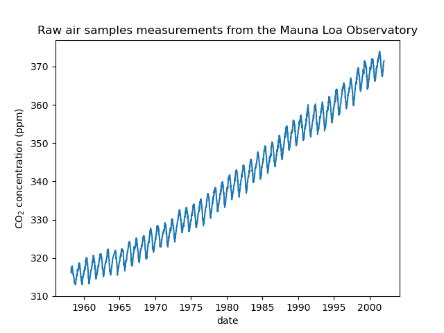
The CO2 concentration are from March, 1958 to December, 2001, which is shown in the plot below.

import matplotlib.pyplot as plt

plt.plot(co2_data["date"], co2_data["co2"])
plt.xlabel("date")
plt.ylabel("CO$_2$ concentration (ppm)")
_ = plt.title("Raw air samples measurements from the Mauna Loa Observatory")

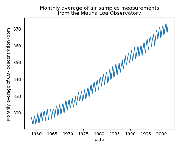
We will preprocess the dataset by taking a monthly average to smooth the data. The months which have no measurements were collected should not be dropped. Because AR models require the time intervals between the two neighboring measurements are consistent. As the results, the NaN values should be kept as the placeholders to maintain the time intervals, and NARX can handle the missing values properly.

co2_data = co2_data.set_index("date").resample("ME")["co2"].mean().reset_index()
plt.plot(co2_data["date"], co2_data["co2"])
plt.xlabel("date")
plt.ylabel("Monthly average of CO$_2$ concentration (ppm)")
_ = plt.title(
    "Monthly average of air samples measurements\nfrom the Mauna Loa Observatory"
)

For plotting, the time axis for training is from March, 1958 to December, 2001, which is converted it into a numeric, e.g., March, 1958 will be converted to 1958.25. The time axis for test is from March, 1958 to nowadays.

import datetime

import numpy as np

today = datetime.datetime.now(tz=datetime.UTC)
current_month = today.year + today.month / 12

x_train = (co2_data["date"].dt.year + co2_data["date"].dt.month / 12).to_numpy()
x_test = np.arange(start=1958.25, stop=current_month, step=1 / 12)

Nonlinear AR model

We can use make_narx() to easily build a nonlinear AR model, which does not has an input. Therefore, the input X is set as None. make_narx() will search 10 polynomial terms, whose maximum degree is 2 and maximum delay is 9.

from fastcan.narx import make_narx, print_narx

max_delay = 9
model = make_narx(
    None,
    co2_data["co2"],
    n_terms_to_select=10,
    max_delay=max_delay,
    poly_degree=2,
    verbose=0,
)
model.fit(None, co2_data["co2"], coef_init="one_step_ahead")
print_narx(model, term_space=27)

| yid |           Term            |   Coef   |
|-----|---------------------------|----------|
|  0  |         Intercept         | -14.881  |
|  0  |       y_hat[k-1,0]        |  1.291   |
|  0  |       y_hat[k-2,0]        |  -0.203  |
|  0  |       y_hat[k-3,0]        |  -0.438  |
|  0  |       y_hat[k-5,0]        |  0.327   |
|  0  |       y_hat[k-8,0]        |  -0.578  |
|  0  |       y_hat[k-9,0]        |  0.688   |
|  0  | y_hat[k-2,0]*y_hat[k-6,0] |  -0.000  |
|  0  | y_hat[k-6,0]*y_hat[k-6,0] |  -0.046  |
|  0  | y_hat[k-6,0]*y_hat[k-7,0] |  0.091   |
|  0  | y_hat[k-7,0]*y_hat[k-7,0] |  -0.046  |

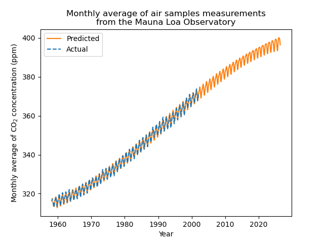
Forecasting performance

As AR model does not require input data, the input X in predict() is used to indicate total steps to forecast. The initial conditions y_init is the first 18 months data from the ground truth, which contains missing values. If there is no missing value given to y_init, we can only use max_delay number of samples as the initial conditions. However, if missing values are given to y_init, NARX will break the data into multiple time series according to the missing values. For each time series, at least max_delay number of samples, which does not have missing values, are required to do the proper forecasting. The results show our fitted model is capable to forecast to future years with only first 18 months data.

y_pred = model.predict(
    len(x_test),
    y_init=co2_data["co2"][:18],
)
plt.plot(x_test, y_pred, label="Predicted", c="tab:orange")
plt.plot(x_train, co2_data["co2"], label="Actual", linestyle="dashed", c="tab:blue")
plt.legend()
plt.xlabel("Year")
plt.ylabel("Monthly average of CO$_2$ concentration (ppm)")
_ = plt.title(
    "Monthly average of air samples measurements\nfrom the Mauna Loa Observatory"
)
plt.show()