Note

Go to the end to download the full example code or to run this example in your browser via JupyterLite.

Computational speed comparison#

In this examples, we will compare the computational speed of three different feature selection methods: h-correlation based FastCan, eta-cosine based FastCan, and baseline model based on sklearn.cross_decomposition.CCA.

# Authors: The fastcan developers
# SPDX-License-Identifier: MIT

Prepare data#

We will generate a random matrix with 3000 samples and 20 variables as feature matrix \(X\) and a random matrix with 3000 samples and 20 variables as target matrix \(y\).

import numpy as np

rng = np.random.default_rng(12345)
X = rng.random((3000, 20))
y = rng.random((3000, 5))

Define baseline method#

The baseline method can be realised by CCA in scikit-learn. The baseline method will, in greedy manner, select the feature which maximizes the canonical correlation between np.column_stack((X_selected, X[:, j])) and y, where X_selected is the selected features in past iterations. As the number of canonical correlation coefficients may be more than one, the feature ranking criterion used here is the sum squared of all canonical correlation coefficients.

from fastcan.utils import ssc


def baseline(X, y, t):
    """Baseline method using CCA from sklearn.

    Parameters
    ----------
    X : array-like of shape (n_samples, n_features)
        Feature matrix.

    y : array-like of shape (n_samples, n_outputs)
        Target matrix.

    t : int
        The parameter is the absolute number of features to select.

    Returns
    -------
    indices_ : ndarray of shape (t,), dtype=int
        The indices of the selected features. The order of the indices
        is corresponding to the feature selection process.

    scores_: ndarray of shape (t,), dtype=float
        The sum of the squared correlation of selected features. The order of
        the scores is corresponding to the feature selection process.
    """
    n_samples, n_features = X.shape
    mask = np.zeros(n_features, dtype=bool)
    r2 = np.zeros(n_features, dtype=float)
    indices = np.zeros(t, dtype=int)
    scores = np.zeros(t, dtype=float)
    X_selected = np.zeros((n_samples, 0), dtype=float)
    for i in range(t):
        for j in range(n_features):
            if not mask[j]:
                X_candidate = np.column_stack((X_selected, X[:, j]))
                r2[j] = ssc(X_candidate, y)
        d = np.argmax(r2)
        indices[i] = d
        scores[i] = r2[d]
        mask[d] = True
        r2[d] = 0
        X_selected = np.column_stack((X_selected, X[:, d]))
    return indices, scores

Elapsed time comparison#

Let the three methods select 10 informative features from the feature matrix \(X\). It can be found that the two FastCan methods are much faster than the baseline method.

from timeit import timeit

import matplotlib.pyplot as plt

from fastcan import FastCan

n_features_to_select = 10

t_h = timeit(
    f"s = FastCan({n_features_to_select}, verbose=0).fit(X, y)",
    number=10,
    globals=globals(),
)
t_eta = timeit(
    f"s = FastCan({n_features_to_select}, eta=True, verbose=0).fit(X, y)",
    number=10,
    globals=globals(),
)
t_base = timeit(
    f"indices, _ = baseline(X, y, {n_features_to_select})", number=10, globals=globals()
)
print(f"Elapsed time using h correlation algorithm: {t_h:.5f} seconds")
print(f"Elapsed time using eta cosine algorithm: {t_eta:.5f} seconds")
print(f"Elapsed time using baseline algorithm: {t_base:.5f} seconds")

Elapsed time using h correlation algorithm: 0.01341 seconds
Elapsed time using eta cosine algorithm: 0.04076 seconds
Elapsed time using baseline algorithm: 6.29354 seconds

Results of selection#

It can be found that the selected indices of the three methods are exactly the same.

r_h = FastCan(n_features_to_select, verbose=0).fit(X, y).indices_
r_eta = FastCan(n_features_to_select, eta=True, verbose=0).fit(X, y).indices_
r_base, _ = baseline(X, y, n_features_to_select)

print("The indices of the selected features:", end="\n")
print(f"h-correlation: {r_h}")
print(f"eta-cosine: {r_eta}")
print(f"Baseline: {r_base}")

The indices of the selected features:
h-correlation: [ 9  5 16  3 17  1  8  0 12 18]
eta-cosine: [ 9  5 16  3 17  1  8  0 12 18]
Baseline: [ 9  5 16  3 17  1  8  0 12 18]

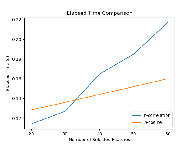
Comparison between h-correlation and eta-cosine methods#

Let’s increase the number of features to 100. Then let the h-correlation method and eta-cosine method to 1 to 30 features and compare their speed performance. There are some interesting findings:

h-correlation method is faster when the number of the selected feature is small.
The slope for eta-cosine method is much lower than h-correlation method.

But why is it? Briefly speaking, at the preprocessing stage, the eta-cosine method requires computing the singular value decomposition (SVD) for np.column_stack((X, y)), which dominates its elapsed time. However, in the following iterated selection process, the eta-cosine method will be much faster than the h-correlation method.

from timeit import repeat

X = rng.random((3000, 400))
y = rng.random((3000, 20))

feature_num = np.arange(20, 61, step=10, dtype=int)


time_h = np.zeros(len(feature_num), dtype=float)
time_eta = np.zeros(len(feature_num), dtype=float)
for i, n_feats in enumerate(feature_num):
    times_h = repeat(
        f"s = FastCan({n_feats + 1}, verbose=0).fit(X, y)",
        number=1,
        repeat=10,
        globals=globals(),
    )
    time_h[i] = np.median(times_h)
    times_eta = repeat(
        f"s = FastCan({n_feats + 1}, eta=True, verbose=0).fit(X, y)",
        number=1,
        repeat=10,
        globals=globals(),
    )
    time_eta[i] = np.median(times_eta)


plt.plot(feature_num, time_h, label="h-correlation")
plt.plot(feature_num, time_eta, label=r"$\eta$-cosine")
plt.title("Elapsed Time Comparison")
plt.xlabel("Number of Selected Features")
plt.ylabel("Elapsed Time (s)")
plt.xticks(feature_num)
plt.legend(loc="lower right")
plt.show()

Total running time of the script: (0 minutes 22.582 seconds)

Gallery generated by Sphinx-Gallery

References

“Canonical-correlation-based fast feature selection for structural health monitoring” Zhang, S., Wang, T., Worden, K., Sun L., & Cross, E. J. Mechanical Systems and Signal Processing, 223:111895 (2025).