Intuitively explanation

Let’s intuitively understand the two methods, h-correlation and eta-cosine, in FastCan.

# Authors: The fastcan developers
# SPDX-License-Identifier: MIT

Select the first feature

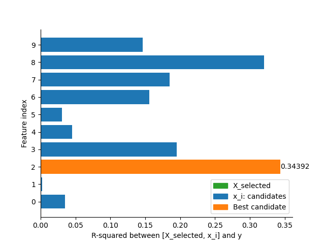
For feature selection, it is normally easy to define a criterion to evaluate a feature’s usefulness, but it is hard to compute the amount of redundancy between a new feature and many selected features. Here we use the diabetes dataset, which has 10 features, as an example. If R-squared between a feature (transformed to the predicted target by a linear regression model) and the target to describe its usefulness, the results are shown in the following figure. It can be seen that Feature 2 is the most useful and Feature 8 is the second. However, does that mean that the total usefulness of Feature 2 + Feature 8 is the sum of their R-squared scores? Probably not, because there may be redundancy between Feature 2 and Feature 8. Actually, what we want is a kind of usefulness score which has the superposition property, so that the usefulness of each feature can be added together without redundancy.

import matplotlib.pyplot as plt
import numpy as np
from matplotlib.patches import Patch
from sklearn.datasets import load_diabetes
from sklearn.linear_model import LinearRegression

from fastcan import FastCan

plt.rcParams["axes.spines.right"] = False
plt.rcParams["axes.spines.top"] = False


def get_r2(feats, target, feats_selected=None):
    """Get R-squared between [feats_selected, feat_i] and target."""

    n_samples, n_features = feats.shape
    if feats_selected is None:
        feats_selected = np.zeros((n_samples, 0))

    lr = LinearRegression()
    r2 = np.zeros(n_features)
    for i in range(n_features):
        feats_i = np.column_stack((feats_selected, feats[:, i]))
        r2[i] = lr.fit(feats_i, target).score(feats_i, target)
    return r2


def plot_bars(ids, r2_left, r2_selected):
    """Plot the relative R-squared with a bar plot."""
    legend_selected = Patch(color="tab:green", label="X_selected")
    legend_cand = Patch(color="tab:blue", label="x_i: candidates")
    legend_best = Patch(color="tab:orange", label="Best candidate")
    n_features = len(ids)
    n_selected = len(r2_selected)

    left = np.zeros(n_features) + sum(r2_selected)
    left_selected = np.cumsum(r2_selected)
    left_selected = np.r_[0, left_selected]
    left_selected = left_selected[:-1]
    left[:n_selected] = left_selected

    label = [""] * n_features
    label[np.argmax(r2_left) + n_selected] = f"{max(r2_left):.5f}"

    colors = ["tab:blue"] * (n_features - n_selected)
    colors[np.argmax(r2_left)] = "tab:orange"
    colors = ["tab:green"] * n_selected + colors

    hbars = plt.barh(ids, width=np.r_[score_selected, r2_left], color=colors, left=left)
    plt.axvline(x=sum(r2_selected), color="tab:orange", linestyle="--")
    plt.bar_label(hbars, label)
    plt.yticks(np.arange(n_features))
    plt.xlabel("R-squared between [X_selected, x_i] and y")
    plt.ylabel("Feature index")
    plt.legend(handles=[legend_selected, legend_cand, legend_best])
    plt.show()


X, y = load_diabetes(return_X_y=True)


id_left = np.arange(X.shape[1])
id_selected = []
score_selected = []


score_0 = get_r2(X, y)

plot_bars(id_left, score_0, score_selected)

Select the second feature

Let’s compute the R-squared between Feature 2 + Feature i and the target, which is shown in the figure below. The bars at the right-hand-side (RHS) of the dashed line is the additional R-squared scores based on the scores of Feature 2, which we call relative usefulness to Feature 2. It is also seen that the bar of Feature 8 in this figure is much shorter than the bar in the previous figure. Because the redundancy between Feature 2 and Feature 8 is removed. Therefore, these bars at RHS can be the desired usefulness score with the superposition property.

index = np.argmax(score_0)
id_selected += [id_left[index]]
score_selected += [score_0[index]]
id_left = np.delete(id_left, index)
score_1 = get_r2(X[:, id_left], y, X[:, id_selected]) - sum(score_selected)


plot_bars(np.r_[id_selected, id_left], score_1, score_selected)

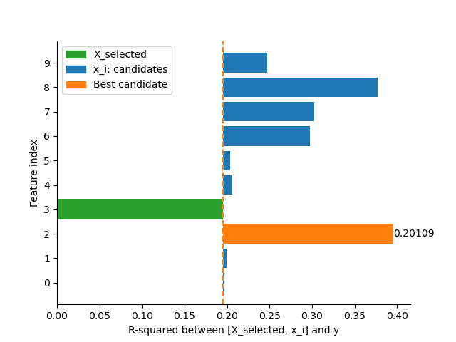
Select the third feature

Again, let’s compute the R-squared between Feature 2 + Feature 8 + Feature i and the target, and the additional R-squared contributed by the rest of the features is shown in following figure. It can be found that after selecting Features 2 and 8, the rest of the features can provide a very limited contribution.

index = np.argmax(score_1)
id_selected += [id_left[index]]
score_selected += [score_1[index]]
id_left = np.delete(id_left, index)
score_2 = get_r2(X[:, id_left], y, X[:, id_selected]) - sum(score_selected)

plot_bars(np.r_[id_selected, id_left], score_2, score_selected)

h-correlation and eta-cosine

h-correlation is a fast way to compute the value of the bars at the RHS of the dashed lines. The fast computational speed is achieved by orthogonalization, which removes the redundancy between the features. We use the orthogonalization first to makes the rest of features orthogonal to the selected features and then compute their additional R-squared values. eta-cosine uses the similar idea, but has an additional preprocessing step to compress the features \(X \in \mathbb{R}^{N\times n}\) and the target \(X \in \mathbb{R}^{N\times n}\) to \(X_c \in \mathbb{R}^{(m+n)\times n}\) and \(Y_c \in \mathbb{R}^{(m+n)\times m}\).

scores = FastCan(3, verbose=0).fit(X, y).scores_

print(f"First selected feature's score: {scores[0]:.5f}")
print(f"Second selected feature's score: {scores[1]:.5f}")
print(f"Third selected feature's score: {scores[2]:.5f}")

First selected feature's score: 0.34392
Second selected feature's score: 0.11556
Third selected feature's score: 0.02060

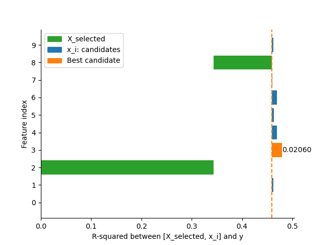
Relative usefulness

The idea about relative usefulness can be very helpful, when we want to evaluate features based on some prior knowledges. For example, we have some magnetic impedance spectroscopy (MIS) features of cervix tissue in pregnant women and we want to evaluate the usefulness of these features for predicting spontaneous preterm births (sPTB). The prior knowledge is that cervical length (CL) and quantitative fetal fibronectin (fFN) are effective risk factors for sPTB, so the redundancy between CL+fFN and MIS features should be avoided. Therefore, the relative usefulness of MIS features to CL and fFN should be computed. We can use the argument indices_include to compute the relative usefulness. Use the diabetes dataset as an example. Assuming the prior knowledge is that Feature 3 is very important, the relative usefulness of the rest features to Feature 3 given in the figure below, which is the same as the result from FastCan.

index = 3
id_selected = [index]
score_selected = [score_0[index]]
id_left = np.arange(X.shape[1])
id_left = np.delete(id_left, index)
score_1_7 = get_r2(X[:, id_left], y, X[:, id_selected]) - sum(score_selected)

plot_bars(np.r_[id_selected, id_left], score_1_7, score_selected)

scores = FastCan(2, indices_include=[3], verbose=0).fit(X, y).scores_

print(f"First selected feature's score: {scores[0]:.5f}")
print(f"Second selected feature's score: {scores[1]:.5f}")

First selected feature's score: 0.19491
Second selected feature's score: 0.20109